---

Time-Fixed Exposure

In this section, we will go through some methods to estimate the average causal effect of a time-fixed treatment / exposure on a specific outcome. We will review binary outcomes, continuous outcomes, and time-to-event data. To follow along with the tutorial, run the following code to set up the data

import numpy as np
import pandas as pd
from lifelines import KaplanMeierFitter

from zepid import load_sample_data, spline, RiskDifference
from zepid.causal.gformula import TimeFixedGFormula, SurvivalGFormula
from zepid.causal.ipw import IPTW, IPMW
from zepid.causal.snm import GEstimationSNM
from zepid.causal.doublyrobust import AIPTW, TMLE

df = load_sample_data(timevary=False)
df = df.drop(columns=['cd4_wk45'])
df[['cd4_rs1', 'cd4_rs2']] = spline(df, 'cd40', n_knots=3, term=2, restricted=True)
df[['age_rs1', 'age_rs2']] = spline(df, 'age0', n_knots=3, term=2, restricted=True)

Which estimator should I use?

What estimator to use is an important question. Unfortunately, my answer is that it depends. Review the following list of estimators to help you decide. Afterwards, I would recommend the following process.

First, what are you trying to estimate? Depending on what you want to estimate (the estimand), some estimators don’t make sense to use. For example, if you wanted to estimate the marginal causal effect comparing all treated versus all untreated, then you wouldn’t want to use g-estimation of structural nested models. G-estimation, as detailed below, targets something slightly different than the target estimand. However, if you were interested in average causal effect within defined strata, then g-estimation would be a good choice. Your causal question can (and should) narrow down the list of potential estimators

Second, does your question of interest require something not available for all methods? This can also narrow down estimators, at least ones currently available. For example, only TimeFixedGFormula, StochasticIPTW, and StochasticTMLE allow for stochastic treatments. See the tutorials on Python for Epidemiologists for further details on what each estimator can do.

Lastly, if there are multiple estimators to use, then use them all. Each has different advantages/disadvantages that don’t necessarily make one unilaterally better than the other. If all the estimators provide similar answers, that can generally be taken as a good sign. It builds some additional confidence in your results. If there are distinctly different results across the estimators, that means that at least one assumption is being substantively broken somewhere. In these situations, I would recommend the doubly robust estimators because they make less restrictive modeling assumptions. Alternatively, machine learning promises to make less restrictive assumptions regarding functional forms. However, the lack of agreement between estimators should be noted.

Binary Outcome

To begin, we are interested in the average causal effect of anti-retroviral therapy (ART) on 45-week risk of death.

\[ACE = \Pr(Y^{a=1}) - \Pr(Y^{a=1})\]

where \(Y^{a}\) indicates the potential outcomes under treatment \(a\). Unfortunately, we cannot observe these potential outcomes (or counterfactuals after they occur). We stuck with our observational data, so we need to make some additional assumptions to go from

\[\Pr(Y | A=1) - \Pr(Y | A=0)\]

to

\[\Pr(Y^{a=1}) - \Pr(Y^{a=1})\]

We will assume conditional mean exchangeability, causal consistency, and positivity. These assumptions allow us to go from our observed data to potential outcomes. See Hernan and Robins for further details on these assumptions and these methods in general. We will assume conditional exchangeability by age (continuous), gender (male / female), baseline CD4 T-cell count (continuous), and baseline detectable viral load (yes / no) throughout. The data set we will use is a simulated data set that comes with zEpid

Our set of confounders for conditional exchangeability is quite large and includes some continuous variables. Therefore, we will use parametric models (for the most part). As a result, we assume that our models are correctly specified, in addition to the above assumptions.

Unadjusted Risk Difference

The first option is the unadjusted risk difference. We can calculate this by

rd = RiskDifference()
rd.fit(df, exposure='art', outcome='dead')
rd.summary()

By using this measure as our average causal effect, we are assuming that there are no confounding variables. However, this is an unreasonable assumption for our observational data. However, the RiskDifference gives us some useful information. In the summary, we find LowerBound and UpperBound. These bounds are the Frechet probability bounds. The true causal effect must be contained within these bounds, without requiring exchangeability. This is a good check. All methods below should produce values that are within these bounds.

Therefore, the Frechet bounds allow for partial identification of the causal effect. We narrowed the range of possible values from two unit width (-1 to 1) to unit width (-0.87 to 0.13). However, we don’t have point identification. The following methods allow for point identification under the assumption of conditional exchangeability.

Our unadjusted estimate is -0.05 (-0.13, 0.04), which we could interpret as: ART is associated with a 4.5% point reduction (95% CL: -0.13, 0.04) in the probability of death at 45-weeks. However, this interpretation implies that ART is given randomly (which is unlikely to occur in the data).

Parametric g-formula

The parametric g-formula allows us to estimate the average causal effect of ART on death by specifying an outcome model. From our outcome model, we predict individuals’ counterfactual outcomes under our treatment plans and marginalize over these predicted counterfactuals. This allows us to estimate the marginal risk under our treatment plan of interest.

To estimate the parametric g-formula, we can use the following code

g = TimeFixedGFormula(df, exposure='art', outcome='dead')
g.outcome_model(model='art + male + age0 + age_rs1 + age_rs2 + cd40 + cd4_rs1 + cd4_rs2 + dvl0')

# Estimating marginal effect under treat-all plan
g.fit(treatment='all')
r_all = g.marginal_outcome

# Estimating marginal effect under treat-none plan
g.fit(treatment='none')
r_none = g.marginal_outcome

riskd = r_all - r_none
print('RD:', riskd)

which gives us an estimated risk difference of -0.076. To calculate confidence intervals, we need to use a bootstrapping procedure. Below is an example that uses bootstrapped confidence limits.

rd_results = []
for i in range(1000):
    s = dfs.sample(n=df.shape[0],replace=True)
    g = TimeFixedGFormula(s,exposure='art',outcome='dead')
    g.outcome_model(model='art + male + age0 + age_rs1 + age_rs2 + cd40 + cd4_rs1 + cd4_rs2 + dvl0',
                    print_results=False)
    g.fit(treatment='all')
    r_all = g.marginal_outcome
    g.fit(treatment='none')
    r_none = g.marginal_outcome
    rd_results.append(r_all - r_none)

se = np.std(rd_results)
print('95% LCL', riskd - 1.96*se)
print('95% UCL', riskd + 1.96*se)

In my run (your results may differ), the estimate’s 95% confidence limits were -0.15, 0.00. We could interpret our results as; the 45-week risk of death when everyone was treated with ART at enrollment was 7.6% points (95% CL: -0.15, -0.00) lower than if no one had been treated with ART at enrollment. For further details and examples of other usage of this estimator see this tutorial

Inverse probability of treatment weights

For the g-formula, we specified the outcome model. Another option is to specify a treatment / exposure model. Specifically, this model predicts the probability of treatment, sometimes called propensity scores. From these propensity scores, we can calculate inverse probability of treatment weights.

Below is some code to calculate our stabilized inverse probability of treatment weights for ART.

iptw = IPTW(df, treatment='art')
iptw.treatment_model('male + age0 + age_rs1 + age_rs2 + cd40 + cd4_rs1 + cd4_rs2 + dvl0',
                     print_results=False)

A variety of diagnostics is available to check the calculated weights. See the below referenced tutorial for further details and examples. For our analysis, we use the following marginal structural model

\[\Pr(Y | A) = \alpha_0 + \alpha_1 A\]

While this model looks like a crude regression model, we are fitting it with the weighted data. The weights make it such that there is no confounding in our pseudo-population. As of v0.8.0, IPTW now estimates the marginal structural model for you. GEE is used to estimate the standard error. Robust standard errors are required since weighting our population builds in some correlation between our observations. We need to account for this. While GEE does account for this, our confidence intervals will be somewhat conservative. Below is code to estimate the marginal structural model and print the results

iptw.marginal_structural_model('art')
iptw.fit()
iptw.summary()

My results were fairly similar to the g-formula (RD = -0.08; 95% CL: -0.16, -0.01). We would interpret this in a similar way: the 45-week risk of death when everyone was treated with ART at enrollment was 8.2% points (95% CL: -0.16, -0.01) lower than if no one had been treated with ART at enrollment.

To account for data that is missing at random, inverse probability of missing weights can be stacked together with IPTW. As of v0.8.0, this is built into the IPTW class. Below is an example with accounting for informative censoring (missing outcome data)

When accounting for censoring by the above variables, a similar is obtained (RD = -0.08, 95% CL: -0.16, -0.01). For further details and examples of other usage of this estimator see this tutorial

Augmented inverse probability weights

As you read through the previous estimators, you may have thought “is there a way to combine these approaches?” The answer is yes! Augmented inverse probability of treatment weights require you to specify both a treatment model (pi-model) and an outcome model (Q-model). But why would you want to specify two models? Well, by specifying both and merging them, AIPTW becomes doubly robust. This means that as long as one model is correct, our estimate will be unbiased on average. Essentially, we get two attempts to get our models correct.

We can calculate the AIPTW estimator through the following code

aipw = AIPTW(df, exposure='art', outcome='dead')

# Treatment model
aipw.exposure_model('male + age0 + age_rs1 + age_rs2 + cd40 + cd4_rs1 + cd4_rs2 + dvl0')

# Outcome model
aipw.outcome_model('art + male + age0 + age_rs1 + age_rs2 + cd40 + cd4_rs1 + cd4_rs2 + dvl0')

# Calculating estimate
aipw.fit()

# Printing summary results
aipw.summary()

In the printed results, we have an estimated risk difference of -0.08 (95% CL: -0.15, -0.02). Confidence intervals come from the efficient influence curve. You can also bootstrap confidence intervals. For the risk ratio, you will need to bootstrap the confidence intervals currently. Our results can be interpreted as: the 45-week risk of death when everyone was treated with ART at enrollment was 8.4% points (95% CL: -0.15, -0.02) lower than if no one had been treated with ART at enrollment.

Similarly, we can also account for missing outcome data using inverse probability weights. Below is an example

aipw = AIPTW(df, exposure='art', outcome='dead')
aipw.exposure_model('male + age0 + age_rs1 + age_rs2 + cd40 + cd4_rs1 + cd4_rs2 + dvl0')
aipw.outcome_model('art + male + age0 + age_rs1 + age_rs2 + cd40 + cd4_rs1 + cd4_rs2 + dvl0')
aipw.missing_model('art + male + age0 + age_rs1 + age_rs2 + cd40 + cd4_rs1 + cd4_rs2 + dvl0')
aipw.fit()
aipw.summary()

AIPTW can also be paired with machine learning algorithms, particularly super-learner. The use of machine learning with AIPTW means we are making less restrictive parametric assumptions than all the model described above. For further details, using super-learner / sklearn with AIPTW, and examples see this tutorial

Targeted maximum likelihood estimation

For AIPTW, we merged IPW and the g-formula. The targeted maximum likelihood estimator (TMLE) is another variation on this procedure. TMLE uses a targeting step to update the estimate of the average causal effect. This approach is doubly robust but keeps some of the nice properties of plug-in estimators (like the g-formula). In general, TMLE will likely have narrower confidence intervals than AIPTW.

Below is code to generate the average causal effect of ART on death using TMLE. Additionally, we will specify a missing outcome data model (like AIPTW and IPTW).

tmle = TMLE(df, exposure='art', outcome='dead')
tmle.exposure_model('male + age0 + age_rs1 + age_rs2 + cd40 + cd4_rs1 + cd4_rs2 + dvl0')
tmle.missing_model('art + male + age0 + cd40 + cd4_rs1 + cd4_rs2 + dvl0')
tmle.outcome_model('male + age0 + age_rs1 + age_rs2 + cd40 + cd4_rs1 + cd4_rs2 + dvl0')
tmle.fit()
tmle.summary()

Using TMLE, we estimate a risk difference of -0.08 (95% CL: -0.15, -0.01). We can interpret this as: the 45-week risk of death when everyone was treated with ART at enrollment was 8.3% points (95% CL: -0.15, -0.01) lower than if no one had been treated with ART at enrollment.

TMLE can also be paired with machine learning algorithms, particularly super-learner. The use of machine learning with TMLE means we are making less restrictive parametric assumptions than all the model described above. For further details, using super-learner / sklearn with TMLE, and examples see this tutorial

Single Cross-fit TMLE

While both AIPTW and TMLE are able to incorporate the use of some machine learning algorithms, there are limits. More specifically, both require that the machine learning algorithms are Donsker. Unfortunately, many flexible algorithms we may want to use may not be Donsker. In this scenario, confidence interval coverage may be below what is expected (i.e. the confidence interval are overly narrow due to over-fitting by the machine learning algorithms).

Recently, cross-fitting procedures have been proposed as a way to weaken this condition. Cross-fitting allows for non-Donsker algorithms. For more extensive details on the cross-fitting procedure and why it is necessary, please see my paper and the references within.

zEpid supports both single and double cross-fitting for AIPTW and TMLE. The following are simple examples that use SuperLearner with a single cross-fitting procedure for TMLE. The 10-fold super-learner consists of a GLM, a step-wise GLM with all first-order interactions, and a Random Forest.

from sklearn.ensemble import RandomForestClassifier
from zepid.superlearner import GLMSL, StepwiseSL, SuperLearner
from zepid.causal.doublyrobust import SingleCrossfitAIPTW, SingleCrossfitTMLE

# SuperLearner setup
labels = ["LogR", "Step.int", "RandFor"]
candidates = [GLMSL(sm.families.family.Binomial()),
              StepwiseSL(sm.families.family.Binomial(), selection="forward", order_interaction=0),
              RandomForestClassifier()]

# Single cross-fit TMLE
sctmle = SingleCrossfitTMLE(df, exposure='art', outcome='dead')
sctmle.exposure_model('male + age0 + age_rs1 + age_rs2 + cd40 + cd4_rs1 + cd4_rs2 + dvl0',
                      SuperLearner(candidates, labels, folds=10, loss_function="nloglik"),
                      bound=0.01)
sctmle.outcome_model('male + age0 + age_rs1 + age_rs2 + cd40 + cd4_rs1 + cd4_rs2 + dvl0',
                     SuperLearner(candidates, labels, folds=10, loss_function="nloglik"))
sctmle.fit()
sctmle.summary()

Using SingleCrossfitTMLE, we estimate a risk difference of -0.08 (95% CL: -0.17, 0.00). We can interpret this as: the 45-week risk of death when everyone was treated with ART at enrollment was 8.3% points (95% CL: -0.17, 0.00) lower than if no one had been treated with ART at enrollment. When comparing SingleCrossfitTMLE to the previous TMLE, you can see the confidence intervals are wider. This is a result of weakening the parametric modeling restrictions (by including the random forest as a possible option in super learner).

As these are new procedures, guidelines on their use are still developing. In my experience, I would recommend at least 100 different partitions to be used. Additionally, the data set must be fairly large (more than 500 observations) to take advantage of the flexibility of the cross-fit estimators with machine learning. If the data set is not that large, I recommend using a higher number of folds with SuperLearner (if using), using single cross-fitting, and using the minimal number of required splits.

G-estimation of SNM

The final method I will review is g-estimation of structural nested mean models (SNM). G-estimation of SNM is distinct from all of the above estimation procedures. The g-formula, IPTW, AIPTW, and TMLE all estimated the average causal effect of ART on mortality comparing everyone treated to everyone untreated. G-estimation of SNM estimate the average causal effect within levels of the confounders, not the average causal effect in the population. Therefore, if no product terms are included in the SNM if there is effect measure modification, then the SNM will be biased due to model misspecification. SNM are useful for learning about effect modification.

To first demonstrate g-estimation, we will assume there is no effect measure modification. For g-estimation, we specify two models; the treatment model and the structural nested model. The treatment model is the same format as the treatment model for IPTW / AIPTW / TMLE. The structural nested model states the interaction effects we are interested in. Since we are assuming no interaction, we only put the treatment variable into the model.

snm = GEstimationSNM(df, exposure='art', outcome='dead')

# Specify treatment model
snm.exposure_model('male + age0 + age_rs1 + age_rs2 + cd40 + cd4_rs1 + cd4_rs2 + dvl0')

# Specify structural nested model
snm.structural_nested_model('art')

# G-estimation
snm.fit()
snm.summary()

psi = snm.psi
print('Psi:', psi)

Similarly, we need to bootstrap our confidence intervals

psi_results = []
for i in range(500):
    dfs = df.sample(n=df.shape[0],replace=True)
    snm = GEstimationSNM(dfs, exposure='art', outcome='dead')
    snm.exposure_model('male + age0 + age_rs1 + age_rs2 + cd40 + cd4_rs1 + cd4_rs2 + dvl0', print_results=False)
    snm.structural_nested_model('art')
    snm.fit()
    psi_results.append(snm.psi)


se = np.std(psi_results)
print('95% LCL', psi - 1.96*se)
print('95% UCL', psi + 1.96*se)

Overall, the SNM results are similar to the other models (RD = -0.09; 95% CL: -0.17, -0.00). Instead, we interpret this estimate as: the 45-week risk of death when everyone was treated with ART at enrollment was 8.8% points (95% CL: -0.17, -0.00) lower than if no one had been treated with ART at enrollment across all strata.

SNM can be expanded to include additional terms. Below is code to do that. For this SNM, we will assess if there is modification by gender

snm = GEstimationSNM(df, exposure='art', outcome='dead')
snm.exposure_model('male + age0 + age_rs1 + age_rs2 + cd40 + cd4_rs1 + cd4_rs2 + dvl0')
snm.structural_nested_model('art + art:male')
snm.fit()
snm.summary()

The 45-week risk of death when everyone was treated with ART at enrollment was 17.6% points lower than if no one had been treated with ART at enrollment, among women. Among men, risk of death with ART treatment at enrollment was 6.8% points lower compared to no treatment.

Remember, g-estimation of SNM is distinct from these other methods and targets a different estimand. It is a great method to consider when you are interested in effect measure modification.

Summary

Below is a figure summarizing the results across methods.

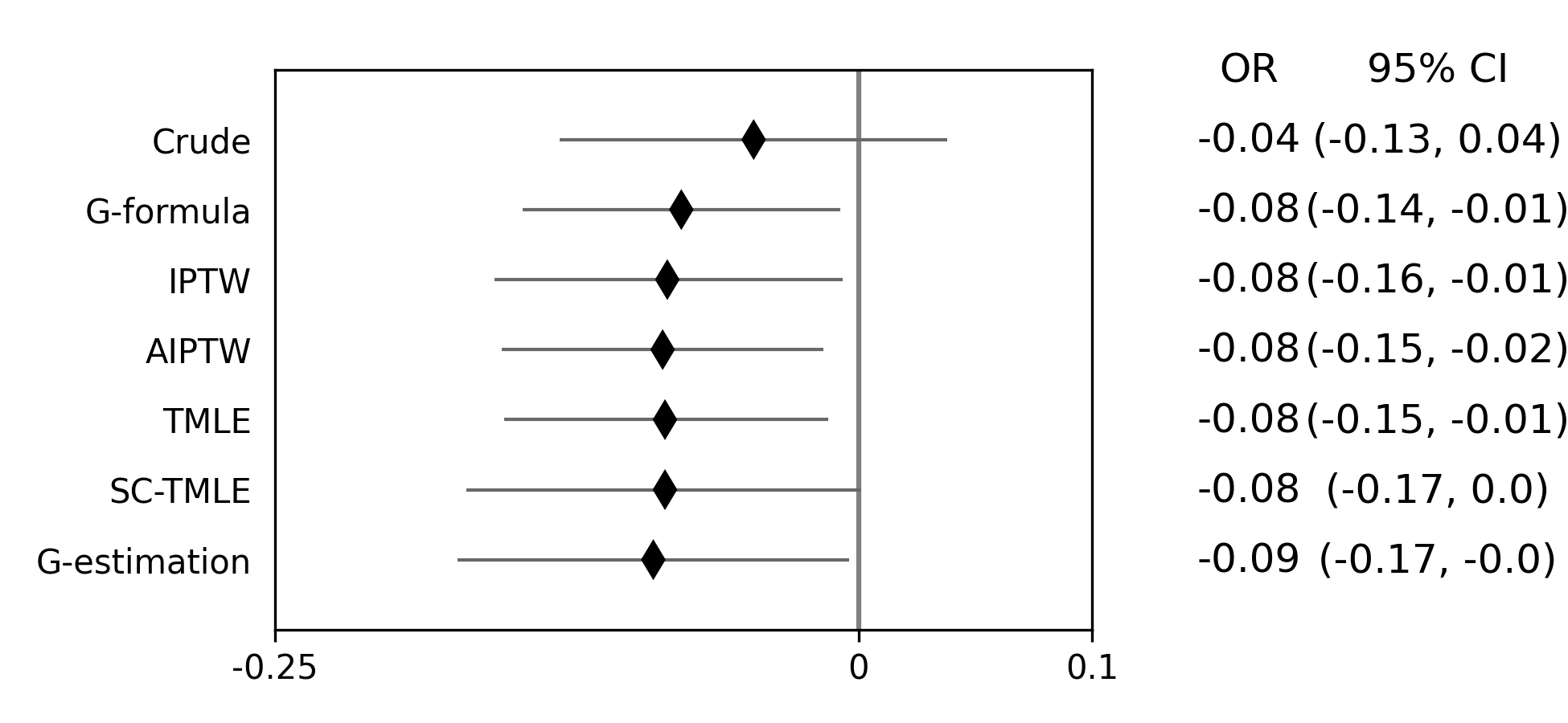
As we can see, all the methods provided fairly similar answers, even the misspecified structural nested model. This will not always be the case. Differences in model results may indicate parametric model misspecification. In those scenarios, it may be preferable to use a doubly-robust estimator with machine learning and cross-fitting (when possible).

Additionally, for simplicity we dropped all missing outcome data. We made the assumption that outcome data was missing completely at random, a strong assumption. We could relax this assumption using built-in methods (e.g. missing_model() functions)

Continuous Outcome

In the previous example we focused on a binary outcome, death. In this example, we will repeat the above procedure but focus on the 45-week CD4 T-cell count. This can be expressed as

\[E[Y^{a=1}] - E[Y^{a=0}]\]

For illustrative purposes, we will ignore the implications of competing risks (those dying before week 45 cannot have a CD4 T-cell count). We will start by restricting our data to only those who are not missing a week 45 T-cell count. In an actual analysis, you wouldn’t want to do this

df = load_sample_data(timevary=False)
dfs = df.drop(columns=['dead']).dropna()

With our data loaded and restricted, let’s compare the estimators. Overall, the estimators are pretty much the same as the binary case. However, we are interested in estimating the average treatment effect instead. Most of the methods auto-detect binary or continuous data in the background. Additionally, we will assume that CD4 T-cell count is appropriately fit by a normal-distribution. Poisson is also available.

Parametric g-formula

The parametric g-formula allows us to estimate the average causal effect of ART on death by specifying an outcome model. From our outcome model, we predict individuals’ counterfactual outcomes under our treatment plans and marginalize over these predicted counterfactuals. This allows us to estimate the marginal risk under our treatment plan of interest.

To estimate the parametric g-formula, we can use the following code

g = TimeFixedGFormula(df, exposure='art', outcome='cd4_wk45', outcome_type='normal')
g.outcome_model(model='art + male + age0 + age_rs1 + age_rs2 + cd40 + cd4_rs1 + cd4_rs2 + dvl0')
g.fit(treatment='all')
r_all = g.marginal_outcome

g.fit(treatment='none')
r_none = g.marginal_outcome
ate = r_all - r_none

print('ATE:', ate)

To calculate confidence intervals, we need to use a bootstrapping procedure. Below is an example that uses bootstrapped confidence limits.

ate_results = []
for i in range(1000):
    s = df.sample(n=df.shape[0],replace=True)
    g = TimeFixedGFormula(s,exposure='art',outcome='cd4_wk45', outcome_type='normal')
    g.outcome_model(model='art + male + age0 + age_rs1 + age_rs2 + cd40 + cd4_rs1 + cd4_rs2 + dvl0',
                    print_results=False)
    g.fit(treatment='all')
    r_all = g.marginal_outcome
    g.fit(treatment='none')
    r_none = g.marginal_outcome
    ate_results.append(r_all - r_none)

se = np.std(ate_results)
print('95% LCL', ate - 1.96*se)
print('95% UCL', ate + 1.96*se)

In my run (your results may differ), the estimate’s 95% confidence limits were 158.70, 370.54. We can interpret this estimate as: the mean 45-week CD4 T-cell count if everyone had been given ART at enrollment was 264.62 (95% CL: 158.70, 370.54) higher than the mean if everyone has not been given ART at baseline.

Inverse probability of treatment weights

Since inverse probability of treatment weights rely on specification of the treatment-model, there is no difference between the weight calculation and the binary outcome. This is also because we assume the same sufficient adjustment set. We will estimate new weights since there is a different missing data pattern. Below is code to estimate our weights

ipw = IPTW(df, treatment='art')
ipw.treatment_model('male + age0 + age_rs1 + age_rs2 + cd40 + cd4_rs1 + cd4_rs2 + dvl0')
ipw.marginal_structural_model('art')
ipw.fit()
ipw.summary()

Our marginal structural model estimates 222.56 (95% CL: 114.67, 330.46). We can interpret this estimate as: the mean 45-week CD4 T-cell count if everyone had been given ART at enrollment was 222.56 (95% CL: 114.67, 330.46) higher than the mean if everyone has not been given ART at baseline.

Augmented inverse probability weights

Similarly to the binary outcome case, AIPTW follows the same recipe to merge IPTW and g-formula estimates. We can calculate the AIPTW estimator through the following code

aipw = AIPTW(df, exposure='art', outcome='cd4_wk45')
aipw.exposure_model('male + age0 + age_rs1 + age_rs2 + cd40 + cd4_rs1 + cd4_rs2 + dvl0')
aipw.outcome_model('art + male + age0 + age_rs1 + age_rs2 + cd40 + cd4_rs1 + cd4_rs2 + dvl0')
aipw.fit()
aipw.summary()

AIPTW produces a similar estimate to the marginal structural model (ATE = 228.22; 95% CL: 115.33, 341.11). We can interpret this estimate as: the mean 45-week CD4 T-cell count if everyone had been given ART at enrollment was 228.22 (95% CL: 115.33, 341.11) higher than the mean if everyone has not been given ART at baseline.

Targeted maximum likelihood estimation

TMLE also supports continuous outcomes and is similarly doubly robust. Below is code to estimate TMLE for a continuous outcome.

tmle = TMLE(df, exposure='art', outcome='cd4_wk45')
tmle.exposure_model('male + age0 + age_rs1 + age_rs2 + cd40 + cd4_rs1 + cd4_rs2 + dvl0')
tmle.outcome_model('art + male + age0 + age_rs1 + age_rs2 + cd40 + cd4_rs1 + cd4_rs2 + dvl0')
tmle.fit()
tmle.summary()

Our results are fairly similar to the other models. The mean 45-week CD4 T-cell count if everyone had been given ART at enrollment was 228.35 (95% CL: 118.97, 337.72) higher than the mean if everyone has not been given ART at baseline.

Single Cross-fit TMLE

Similarly, we can pair TMLE with a cross-fitting procedure and machine learning. In this example, we use SuperLearner with a GLM, a stepwise selection, and a random forest.

from sklearn.ensemble import RandomForestClassifier, RandomForestRegressor

# SuperLearner set-up
labels = ["LogR", "Step.int", "RandFor"]
b_candidates = [GLMSL(sm.families.family.Binomial()),
                StepwiseSL(sm.families.family.Binomial(), selection="forward", order_interaction=0),
                RandomForestClassifier(random_state=809512)]
c_candidates = [GLMSL(sm.families.family.Gaussian()),
                StepwiseSL(sm.families.family.Gaussian(), selection="forward", order_interaction=0),
                RandomForestRegressor(random_state=809512)]

# Single cross-fit TMLE
sctmle = SingleCrossfitTMLE(df, exposure='art', outcome='cd4_wk45')
sctmle.exposure_model('male + age0 + age_rs1 + age_rs2 + cd40 + cd4_rs1 + cd4_rs2 + dvl0',
                      SuperLearner(b_candidates, labels, folds=10, loss_function="nloglik"),
                      bound=0.01)
sctmle.outcome_model('male + age0 + age_rs1 + age_rs2 + cd40 + cd4_rs1 + cd4_rs2 + dvl0',
                     SuperLearner(c_candidates, labels, folds=10))
sctmle.fit(n_partitions=3, random_state=201820)
sctmle.summary()

The mean 45-week CD4 T-cell count if everyone had been given ART at enrollment was 176.9 (95% CL: -37.7, 391.5) higher than the mean if everyone has not been given ART at baseline.

The point estimate is similar to other approaches, but the confidence intervals are substantially wider. This is likely a result of the random forest dominating super-learner and being somewhat dependent on the particular split. This is the penalty of weaker modeling assumptions (or rather it showcases the undue confidence that results from assuming that our particular parametric model is sufficient in other estimators).

G-estimation of SNM

Recall that g-estimation of SNM estimates the average causal effect within levels of the confounders, not the average causal effect in the population. Therefore, if no product terms are included in the SNM if there is effect measure modification, then the SNM will be biased due to model misspecification.

For illustrative purposes, I will specify a one-parameter SNM. Below is code to estimate the model

snm = GEstimationSNM(df, exposure='art', outcome='cd4_wk45')
snm.exposure_model('male + age0 + age_rs1 + age_rs2 + cd40 + cd4_rs1 + cd4_rs2 + dvl0')
snm.structural_nested_model('art')
snm.fit()
snm.summary()

Overall, the SNM results are similar to the other models (ATE = 227.2). Instead, we interpret this estimate as: the mean 45-week CD T-cell count when everyone was treated with ART at enrollment was 227.2 higher (95% CL: 134.2, 320.2) than if no one had been treated with ART at enrollment across all strata.

SNM can be expanded to include additional terms. Below is code to do that. For this SNM, we will assess if there is modification by gender

snm = GEstimationSNM(df, exposure='art', outcome='cd4_wk45')
snm.exposure_model('male + age0 + age_rs1 + age_rs2 + cd40 + cd4_rs1 + cd4_rs2 + dvl0')
snm.structural_nested_model('art + art:male')
snm.fit()
snm.summary()

The mean 45-week CD4 T-cell count when everyone was treated with ART at enrollment was 277.1 higher than if no one had been treated with ART at enrollment, among women. Among men, CD4 T-cell count with ART treatment at enrollment was 213.8 higher compared to no treatment.

Remember, g-estimation of SNM is distinct from these other methods and targets a different estimand. It is a great method to consider when you are interested in effect measure modification.

Summary

Below is a figure summarizing the results across methods.

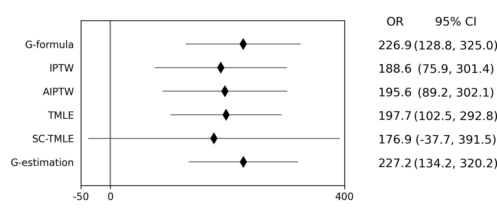
There was some difference in results between outcome models and treatment models. Specifically, the g-formula and IPTW differ. AIPTW and TMLE are similar to IPTW. This may indicate substantive misspecification of the outcome model. This highlights why you may consider using multiple models.

Additionally, for simplicity we dropped all missing outcome data. We made the assumption that outcome data was missing complete at random, a strong assumption. We could relax this assumption by pairing the above methods with inverse-probability-of-missing-weights or using built-in methods (like TMLE’s missing_model)

Causal Survival Analysis

Previously, we focused on the risk of death at 45-weeks. However, we may be interested in conducting a time-to-event analysis. For the following methods, we will focus on treatment at baseline. Specifically, we will not allow the treatment to vary over time. For methods that allow for time-varying treatment, see the tutorial for time-varying exposures.

For the following analysis, we are interested in the average causal effect of ART treatment at baseline compared to no treatment. We will compare the parametric g-formula and IPTW. The parametric g-formula is further described in Hernan’s “The hazards of hazard ratio” paper. For the analysis in this section, we will get a little help from the lifelines library. It is a great library with a variety of survival models and procedures. We will use the KaplanMeierFitter function to estimate risk function

Parametric g-formula

We can use a similar g-formula procedure to estimate average causal effects with time-to-event data. To do this, we use a pooled logistic model. We then use the pooled logistic regression model to predict outcomes at each time under the treatment strategy of interest. For the pooled logistic model, it is fit to data in a long format, where each row corresponds to one unit of time per participant. There will be multiple rows per participant.

For SurvivalGFormula, we need to convert the data set into a long format. We can do that with the following code

df = load_sample_data(False).drop(columns=['cd4_wk45'])
df['t'] = np.round(df['t']).astype(int)
df = pd.DataFrame(np.repeat(df.values, df['t'], axis=0), columns=df.columns)
df['t'] = df.groupby('id')['t'].cumcount() + 1
df.loc[((df['dead'] == 1) & (df['id'] != df['id'].shift(-1))), 'd'] = 1
df['d'] = df['d'].fillna(0)

# Spline terms
df[['t_rs1', 't_rs2', 't_rs3']] = spline(df, 't', n_knots=4, term=2, restricted=True)
df[['cd4_rs1', 'cd4_rs2']] = spline(df, 'cd40', n_knots=3, term=2, restricted=True)
df[['age_rs1', 'age_rs2']] = spline(df, 'age0', n_knots=3, term=2, restricted=True)

If you look at this data, you will notice there are multiple rows per participant. Each row for a participant corresponds to one unit of time (weeks in this example) up to the event time or 45-weeks. All variables (aside from time and outcomes) take the same value over follow-up. This is because we are interested in the baseline exposure. We then adjust for all baseline confounders. Nothing should be time-varying in this model (aside from the outcome and time).

We can estimate the average causal effect comparing a treat-all plan versus a treat-none. Below is code to estimate the time-to-event g-formula

sgf = SurvivalGFormula(df.drop(columns=['dead']), idvar='id', exposure='art', outcome='d', time='t')
sgf.outcome_model(model='art + male + age0 + age_rs1 + age_rs2 + cd40 + '
                        'cd4_rs1 + cd4_rs2 + dvl0 + t + t_rs1 + t_rs2 + t_rs3')
sgf.fit(treatment='all')
sgf.plot(c='b')

sgf.fit(treatment='none')
sgf.plot(c='r')
plt.ylabel('Probability of death')
plt.show()

The plot functionality will return the following plot of the cumulative incidence function

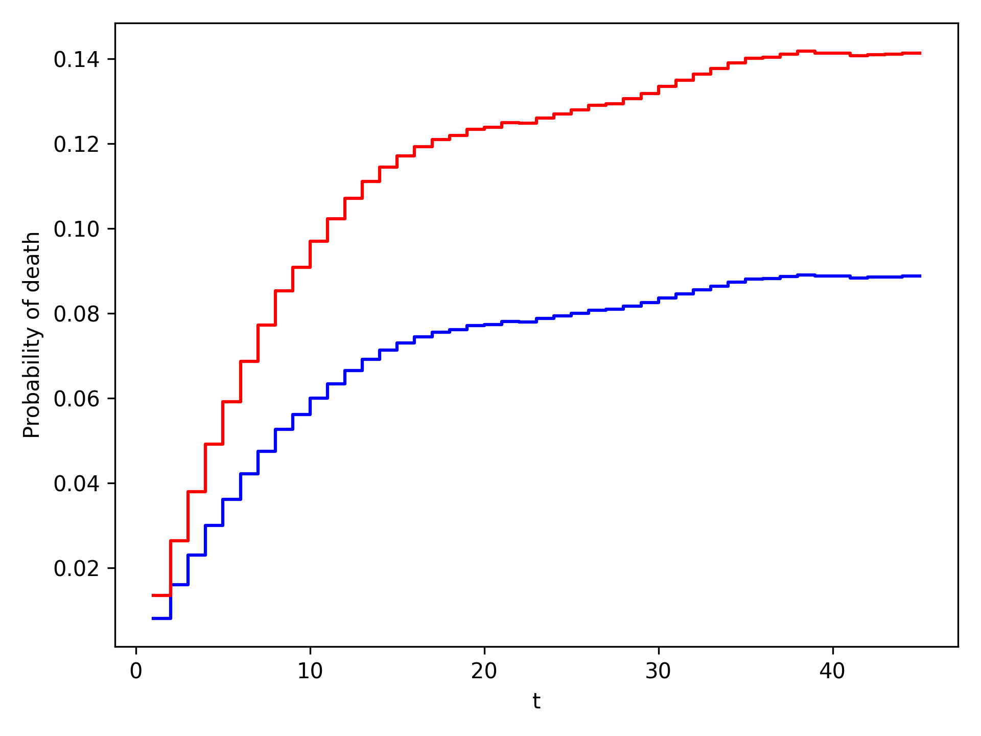
We see that ART reduces mortality throughout follow-up

Inverse probability of treatment weights

A new estimator, SurvivalIPTW will soon be implemented and available to estimate IPTW-adjusted survival curves.

Summary

Currently, only these two options are available. I plan on adding further functionalities in future updates

The difference in these results highlight the differences between the approaches. The g-formula makes some strong parametric assumptions, but smooths over sparse data. IPTW uses the observed data, so it is more sensitive to sparse data. IPTW particularly highlights why we might consider using methods to handle time-varying treatments. Particularly, if few participants are treated at baseline, then we may have trouble estimating the average causal effect. Please refer to the Time-Varying Treatment tutorial for further discussion.